Share article
Identifying ants with object detection and classification models
Introduction
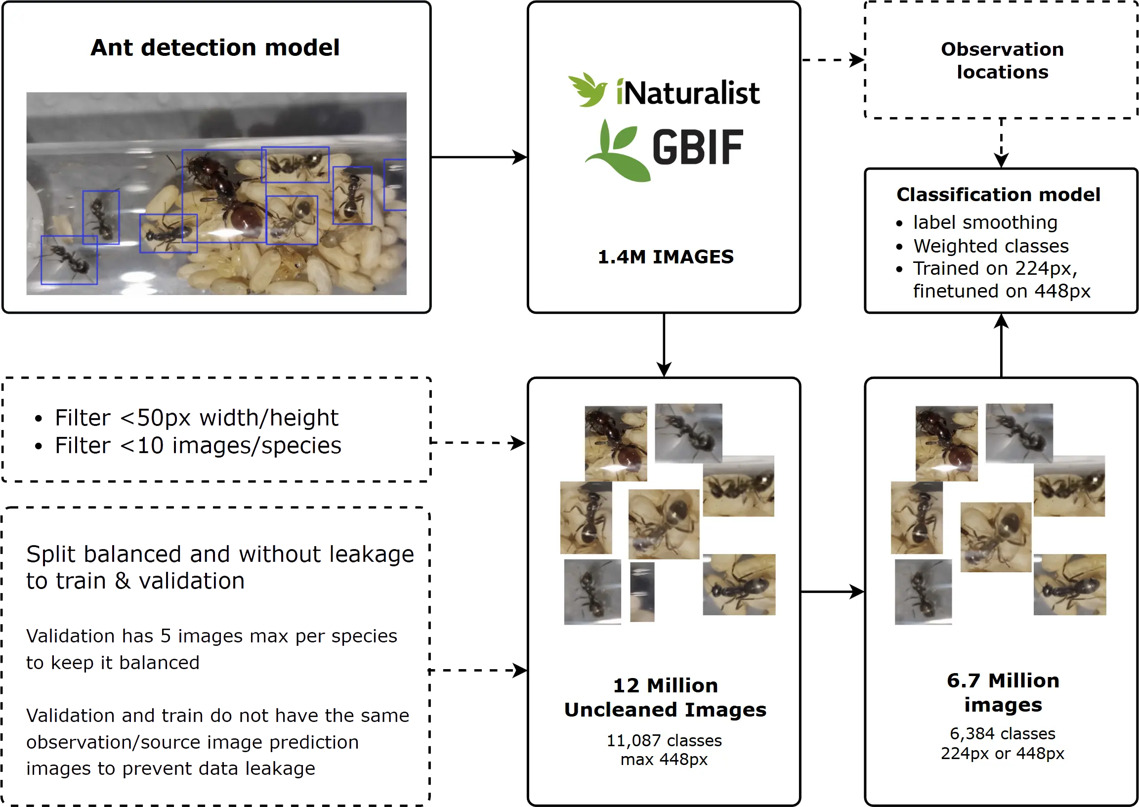
My goal with AntScout is to build the world’s most accurate ant identification system. While most standard models try to classify an entire image at once, I’ve found that a specialized two-stage pipeline using object detection to isolate individual ants before classification, delivers significantly better results. By focusing the classification model entirely on fine-grained anatomical details of cropped ants, we can better distinguish between the 13,000+ species that often look identical to the naked eye.
Through this project, I’m leveraging over 1.5 million images from iNaturalist and GBIF in combination with DINOv3 and ecological data to push the boundaries of what’s possible in automated entomology.
Step 1: Object Detection
Finding the ants within the image is the foundation. I use a specialized object detection model to locate each ant, which is then cropped and sent to the classification model. For a deep dive into the benchmarks and architecture decisions for this phase (including YOLOv11 and RF-DETR), check out the dedicated post Choosing and training the best object detection model for ants.
Technical Architecture
I chose DINOv3 ViT-L/16 as my backbone. Vision transformers like DINOv3 output several components: a CLS token (a global representation of the entire image) and patch tokens (local representations of specific image regions).
To reach the highest possible accuracy, I designed a custom model head that leverages both:
1. Location & Habitat Encoding
The location input goes far beyond simple coordinates. I use a combination of spatial and ecological data to give the model a complete “sense of place”:
- Fourier Features: Latitude and longitude are encoded using Fourier features, which helps the model learn periodic spatial patterns and prevents it from over-focusing on exact GPS points.
- Ecological Context (40+ Layers): Using high-resolution global maps, I sample over 40 distinct habitat variables for every observation:
- Land Cover: Consensus classes from EarthEnv (e.g., evergreen forest, cultivated land, open water).
- Climate (BioClim): 19 variables from WorldClim, including temperature seasonality, annual precipitation, and coldest quarter mean temperature.
- Soil Chemistry (SoilGrids): 10 layers describing the ground itself, such as pH level, nitrogen content, and sand/clay/silt ratios, crucial for ground-nesting ants.
- Topography: Accurate elevation data to differentiate between lowland and alpine specialists.
This modular location embedding is then used to generate FiLM (Feature-wise Linear Modulation) parameters. These parameters modulate the visual features from DINOv3, essentially telling the model: “This image is from a high-latitude, acidic-soil forest in Scandinavia, look for Formica or Myrmica traits.” A film_scale of 0.7 balances visual evidence with geographical probability.
2. Dual Pooling Strategy
The model combines two ways of summarizing the image:
- CLS Token: DINOv3’s global representation.
- GeM Pooling: Generalized Mean pooling over all patch tokens, which learns to balance between average and max pooling (learned power of ~1.34).
These vectors are concatenated with the location embedding into a combined 3072-dim feature vector, which passes through a wide bottleneck (8192 → 4096) with Squeeze-and-Excitation (SE) attention to learn channel importance.
3. Taxonomic Classification Heads
The final 4096-dim embedding feeds into multiple classification heads sharing the same representation:
- Species: ArcFace layer (~6500 classes)
- Genus: Linear layer (~450 classes)
- Tribe: Linear layer (~120 classes)
- Subfamily: Linear layer (~12 classes)
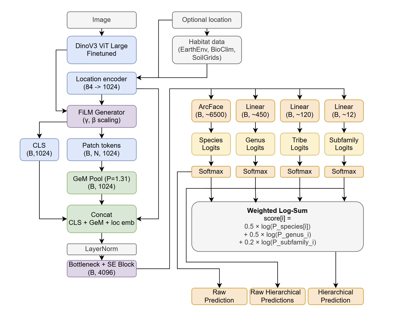
4. Aggregated Scoring
At inference time, I use an Additive Log-Prob fusion method that combines probabilities from all heads. This “anchors” the identification; if the species head is uncertain, the 99% confident genus head ensures the final prediction stays within the correct taxonomic group.
Normalized Classification (ArcFace vs Softmax)
To handle 6500+ species, I used ArcFace instead of standard Softmax. Softmax can allow common classes to develop “louder” weight vectors simply by having more data, making rare species harder to classify. ArcFace solves this by L2-normalizing both features and class weights, ensuring classification is based purely on the angle between a sample and its class center.
I also experimented with the Margin (m) parameter, which pushes classes further apart to improve separation:
| Setting | Val (Loc) | Val (NoLoc) | AntScout (Loc) | AntScout (NoLoc) |
|---|---|---|---|---|
| m=0 (No Margin) | 69.37% | 57.10% | 63.35% | 41.95% |
| m=0.1 Fixed | 69.91% | 57.53% | 61.97% | 40.08% |
| m=0.02-0.15 Adaptive | 69.91% | 57.48% | 61.93% | 40.10% |
Conclusion: While a margin helps on the perfectly balanced validation set, it causes “over-confidence” that hurts performance on the realistically balanced AntScout dataset. The final model uses m=0 (also known as CosFace with no margin), which keeps all species on an equal footing while maintaining better calibration for field photos.
To push accuracy to the limit, I moved beyond standard Cross-Entropy loss:
- PRA Loss (Patch-Relevant Attention): This custom loss implements Hard-Negative Mining. During training, the model is forced to differentiate between “hard negatives”, different species from the same genus. This forces the Siamese-style architecture to learn the tiny anatomical differences (like the shape of a propodeal spine or the length of a scape) that separate closely related species.
- Koleo Loss: Adopted from the original DINO research, this loss encourages a uniform spread of embeddings across the hypersphere, preventing “mode collapse” where different species might cluster too closely together.
- Gram Anchoring: This loss maintains structural consistency by comparing the Gram matrices (pairwise similarities) of patch tokens between the student model and the teacher (EMA) model, ensuring that the spatial understanding stays stable during fine-tuning.
Training Configuration
- Hardware: 2x RTX PRO 6000 WS (96GB VRAM each), later with FP8: 4x RTX 5090 (32GB VRAM each)
- Strategy: Maximum 1000 images per class per epoch to prevent overfitting and speed up training (2 hours/epoch at 448px).
- FP8 Training: Leveraging torchao, the backbone is trained in FP8 precision. This significantly boosts throughput and allows for larger batch sizes on modern Ada Lovelace GPUs while maintaining identification accuracy.
- LLRD (Layer-wise Learning Rate Decay): The 24 transformer blocks of the ViT-L backbone use decaying learning rates. This ensures that the early layers (which learn general features) stay relatively stable while the later layers can adapt more aggressively to the specifics of ant anatomy. LLRD of 0.98 seemed to be most optimal.
- Backbone: DINOv3 ViT-L/16 unfrozen after 2 epochs. The backbone had very low accuracy when unfrozen, this could also have been unfrozen right away.
Training Results: Class Balancing
Optimal results were achieved using a Beta of 0.99 and a max weight of 20x for initial training, followed by fine-tuning with a more aggressive 1000x max ratio. This two-stage approach ensures the model learns both rare and common species effectively.
Training Evolution:
- DINOV3 V1: Linear head using only the CLS token, no EMA.
- DINOV3 V2: Added GeM pooling and a Conv2D layer; unfrozen after epoch 11 with progressive balancing.
- DINOV3 V3: Refined dual-pooling (CLS + GeM) and habitat-aware FiLM conditioning. Optimized with a two-stage LR strategy (0.001 → 0.0002).
Note on training: I’ve found that the use of a correct EMA is extremely important. It helps especially with higher learning rates. Higher learning rate this way gets a higher accuracy than lower learning rate, but this gives worse accuracy on out of distribution data, and degrades on both when then switching to a lower learning rate. Best is to use 0.001 learning rate, then eventually fine tune it with 0.0002, even if the accuracy on the validation set decreases. Going lower than 0.0002 degrades accuracy. Training too long on 0.001 learning rate seems to only degrade the out of distribution AntScout dataset. Having the out of distribution dataset here really helps get a better understanding while training. I used AdamW + Lookahead (which helped convergence speed) with weight decay 0.2 for the head and 0.04 for the backbone.
Final evaluation results
Validation set without location data
| Model | Top-1 Species Accuracy | Top-5 Species Accuracy | Top-1 Genus Accuracy | Top-5 Genus Accuracy | Resolution |
|---|---|---|---|---|---|
| DINOv3 ViT-L/16 V3 | 57.03% | 81.59% | 93.53% | 98.73% | 448px |
| DINOv3 ViT-L/16 V3 HIER | 57.08% | 82.08% | - | - | 448px |
| DINOv3 ViT-L/16 V3 TTA | 57.43% | 81.81% | 93.60% | 98.78% | 448px |
| DINOv3 ViT-L/16 V3 TTA HIER | 57.39% | 82.18% | - | - | 448px |
| DINOv3 ViT-L/16 V2 | 51.24% | 75.38% | 90.43% | 97.05% | 448px |
Validation set with location data
| Model | Top-1 Species Accuracy | Top-5 Species Accuracy | Top-1 Genus Accuracy | Top-5 Genus Accuracy | Resolution |
|---|---|---|---|---|---|
| DINOv3 ViT-L/16 V3 | 69.37% | 89.82% | 95.59% | 99.28% | 448px |
| DINOv3 ViT-L/16 V3 HIER | 69.43% | 90.00% | - | - | 448px |
| DINOv3 ViT-L/16 V3 TTA | 69.55% | 89.87% | 95.60% | 99.27% | 448px |
| DINOv3 ViT-L/16 V3 TTA HIER | 69.57% | 89.99% | - | - | 448px |
| DINOv3 ViT-L/16 V2 | 61.15% | 84.57% | 92.76% | 98.15% | 448px |
(Uncleaned) AntScout set with location data
| Model | Top-1 Species Accuracy | Top-5 Species Accuracy | Top-1 Genus Accuracy | Top-5 Genus Accuracy | Resolution |
|---|---|---|---|---|---|
| DINOv3 ViT-L/16 V3 | 64.37% | 93.30% | 93.89% | 98.97% | 448px |
| DINOv3 ViT-L/16 V3 HIER | 65.00% | 93.06% | - | - | 448px |
| DINOv3 ViT-L/16 V3 TTA | 64.40% | 93.42% | 94.19% | 99.06% | 448px |
| DINOv3 ViT-L/16 V3 TTA HIER | 64.89% | 93.40% | - | - | 448px |
| DINOv3 ViT-L/16 V2 | 63.83% | - | - | - | 448px |
(Uncleaned) AntScout set without location data
| Model | Top-1 Species Accuracy | Top-5 Species Accuracy | Top-1 Genus Accuracy | Top-5 Genus Accuracy | Resolution |
|---|---|---|---|---|---|
| DINOv3 ViT-L/16 V3 | 42.18% | 76.63% | 83.61% | 95.71% | 448px |
| DINOv3 ViT-L/16 V3 HIER | 42.70% | 77.59% | - | - | 448px |
| DINOv3 ViT-L/16 V3 TTA | 42.78% | 76.95% | 84.25% | 95.78% | 448px |
| DINOv3 ViT-L/16 V3 TTA HIER | 43.59% | 78.13% | - | - | 448px |
| DINOv3 ViT-L/16 V2 | 36.99% | - | - | - | 448px |
Note on Logit Adjustment: The chart above shows the impact of the Tau (τ) parameter on balanced vs. realistic datasets. Increasing τ pushes the model to be more conservative on rare species, effectively “out-balancing” the predictions to favor either the AntScout realistic distribution or the perfectly balanced validation set.
Benchmarking against iNaturalist
Comparing localized models is difficult, as pipeline architectures vary. To make this comparison fair, I upload full images to both models. My pipeline detects and classifies up to 10 ants individually, while other models classify the entire image as one.
Because the evaluation set is challenging for general-purpose models, I used common species they are trained on. All test images were unseen by both models during training.
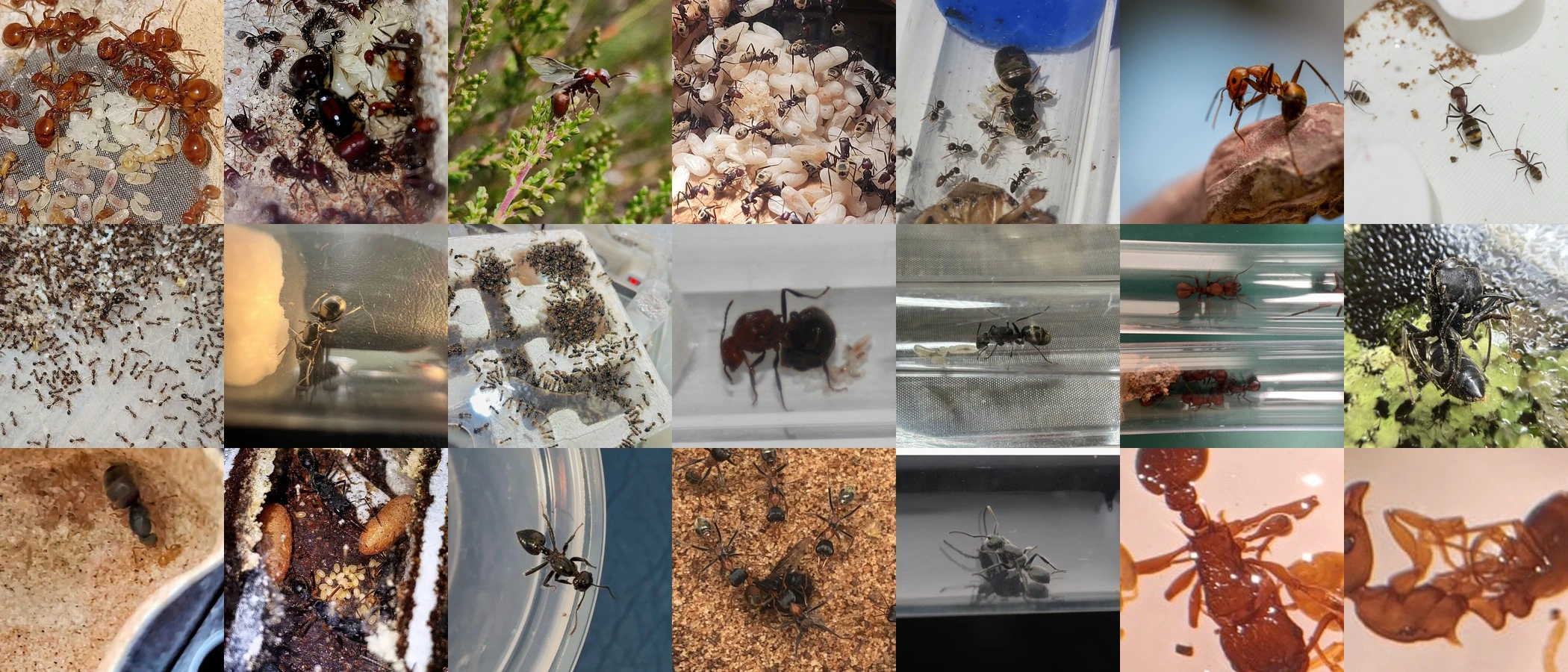
The evaluation dataset for this is quite small as I need to manually run inference on them via inaturalist. The evaluation set used for this can be seen in the header image of this blog post.
Scoring system
Its a really simples scoring system, it just gets either one of these 4 options, or none at all. Then after its done, I just sum up the points for each model. I will also remove all where they both got it fully correct, to only see where they differ.
| Prediction | Rank | Points |
|---|---|---|
| Exact Species | 1st Option | 14 |
| Correct genus | 1st option | 8 |
| Correct Tribes | 1st Option | 4 |
| Correct Subfamily | 1st Option | 2 |
Browse Individual Predictions
Examples
Example why hierarchial weighting is beneficial
This example shows how a standard model can easily get ‘lost’ in the visual details of similar species. However, by using hierarchical weighting, the model leverages its high confidence in the Subfamily (74.69%) and Genus (50.87%) to ‘anchor’ the prediction.
2. Philidris (0.47%)
3. Dolichoderus_diversus (0.43%)
4. Azteca_mayrii (0.36%)
5. Cryptopone (0.29%)
2. Azteca_xanthochroa (3.44%)
3. Azteca_instabilis (3.21%)
4. Azteca (3.18%)
5. Azteca_isthmica (3.11%)
Tribe: Leptomyrmecini (74.37%)
Genus: Azteca (50.87%)
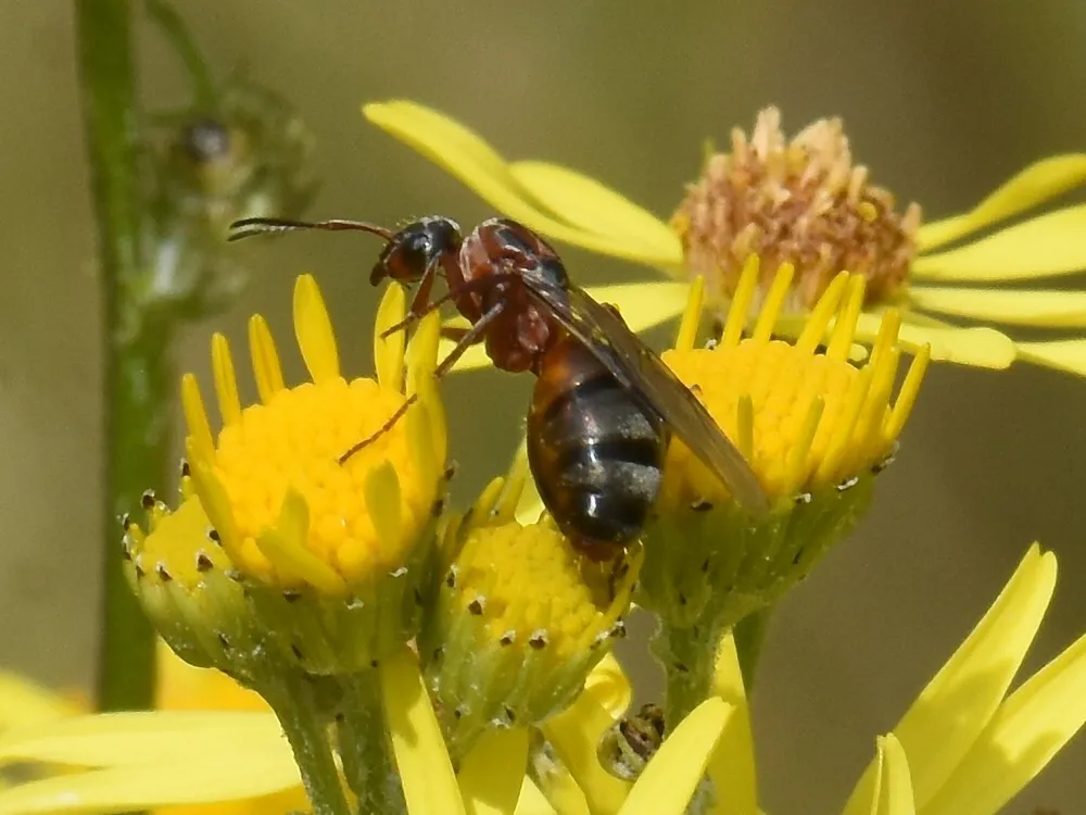
Examples on rare species
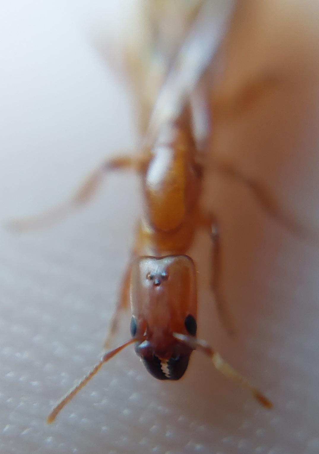
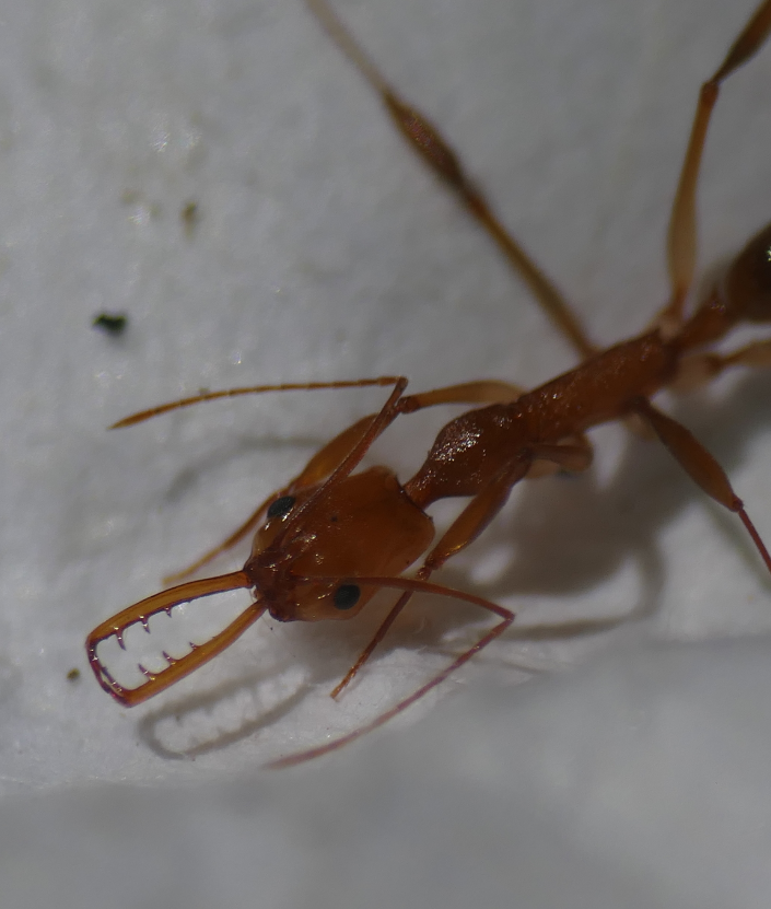
Identification of rare species is one of the biggest challenges in entomology. This Anochetus horridus example is particularly impressive because the model was trained exclusively on pinned specimen images. Despite the shift from high-resolution, professional lab equipment to real-world field photography with natural lighting and complex backgrounds, the model successfully generalized its learned features to correctly identify the genus and species.
2. Anochetus_horridus (0.79%)
3. Anochetus (0.68%)
4. Anochetus_emarginatus (0.66%)
5. Anochetus_mayri (0.61%)
2. Anochetus_horridus (8.68%)
3. Anochetus (8.09%)
4. Anochetus_emarginatus (7.96%)
5. Anochetus_mayri (7.66%)
Tribe: Ponerini (95.23%)
Genus: Anochetus (97.28%)
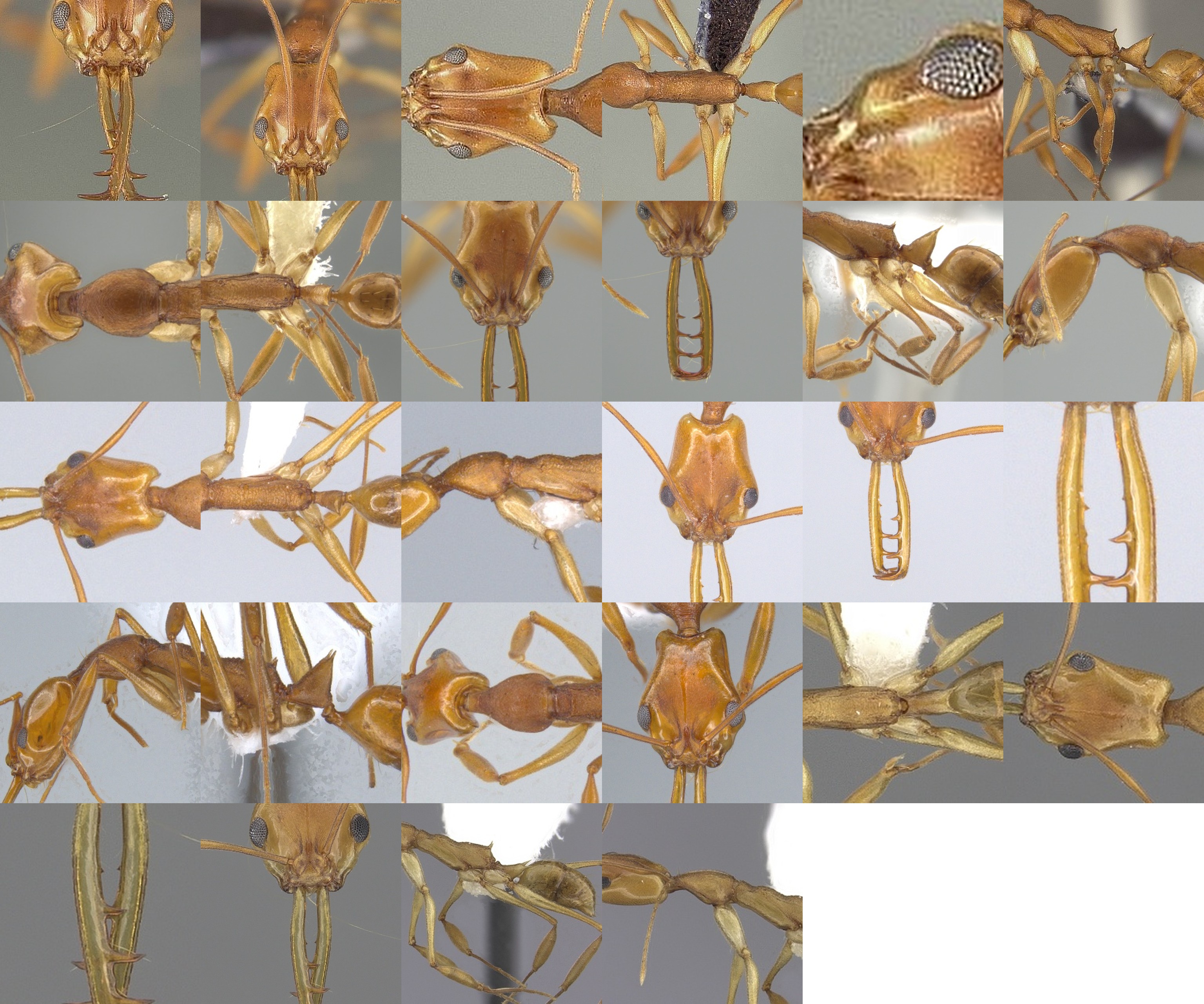
The Anochetus horridus is way more impressive than you would think. This species was only trained on specimen images! Heres all the images it was trained on

2. Anochetus_micans (0.65%)
3. Anochetus_inermis (0.58%)
4. Anochetus_horridus (0.51%)
5. Anochetus_diegensis (0.35%)
2. Anochetus_micans (7.92%)
3. Anochetus_inermis (7.44%)
4. Anochetus_horridus (6.99%)
5. Anochetus_diegensis (5.79%)
Tribe: Ponerini (93.46%)
Genus: Anochetus (98.26%)
2. Pachycondyla_crassinoda (1.54%)
3. Dinoponera_grandis (0.58%)
4. Pachycondyla (0.47%)
5. Ectomomyrmex_astutus (0.38%)
2. Pachycondyla_crassinoda (6.16%)
3. Pachycondyla (3.40%)
4. Pachycondyla_striata (2.53%)
5. Pachycondyla_fuscoatra (2.49%)
Tribe: Ponerini (97.82%)
Genus: Paltothyreus (51.31%)
2. Myrmica_sulcinodis (1.29%)
3. Myrmica_punctiventris (1.10%)
4. Myrmica (0.77%)
5. Myrmicini (0.60%)
2. Myrmica_sulcinodis (11.05%)
3. Myrmica_punctiventris (10.22%)
4. Myrmica (8.54%)
5. Myrmica_scabrinodis (7.03%)
Tribe: Myrmicini (96.94%)
Genus: Myrmica (96.98%)
Conclusion
This project has demonstrated that a specialized pipeline separating object detection from classification can significantly outperform general-purpose models for ant identification. By leveraging the self-supervised learning capabilities of DINOv3, implementing a custom hierarchical loss function, and integrating geographical data, I was able to create a model that is not only accurate but also robust across different resolutions and scenarios.
The comparison with iNaturalist highlights the strength of this approach, particularly in cases where location data is missing or when dealing with challenging images. While the current results are promising, the field of computer vision is moving fast. Future improvements could involve expanding the dataset with even more diverse sources, refining the class balancing techniques, or experimenting with larger model architectures. For now, however, this model stands as a powerful tool for the ant keeping community, pushing the boundaries of what’s possible in automated species identification.
Possible improvements and future work
- Use different backbones like DINOv3 7B, which requires more memory but are expected to perform better. In testing, the huge version already performed significantly better on the AntScout and slightly on the validation, compared to the Large version, which means it generalizes better and works better in real world, out of distribution scenarios.
- Further improve the hierarchical loss function and logic.
- Use a better object detection model to get a better quality dataset. For example using DINOv3 instead of yolo, combined with DETR or Co DETR which gets SOTA results, which then in return also boosts this model. Also using a more reliable crop of the ants, fully covering the antenna and legs.
- Use wider crops to also make it use antenna and legs more often.
- Use higher resolution images to get even more details.
- Use more data and higher quality data. Ideas are for example to filter out outliars based on location or current model.
- Only use research grade images for high quantity species, to reduce the amount of noise in the dataset.
Leave a Comment